All calculating implementations you already can find at our github!

Data Collection

Our dataset consists of 41 clips and contains:

• 28 movie fragment clips
• 10 sport stream clips
• 3 live caption clips

The resolution of our clips is 1920×1080.
The duration of the clips is from 13 to 38 seconds.

50 observers (19–24 y. o.) watched each video with cross-fade by adding a black frame between scenes in free-view task mode and the eye-tracker collected their fixations. Cross-fade ensures the independence of the received fixations between different clips. The SMI iViewXTM Hi-Speed 1250 with a frequency of 500 Hz (~20 fixations per frame) was used.

The final ground-truth saliency map was estimated as a Gaussian mixture with centers at the fixation points. A standard deviation for the Gaussians equal to 120 was chosen (this value matches 8 angular degrees, which is known to be the sector of sharp vision).

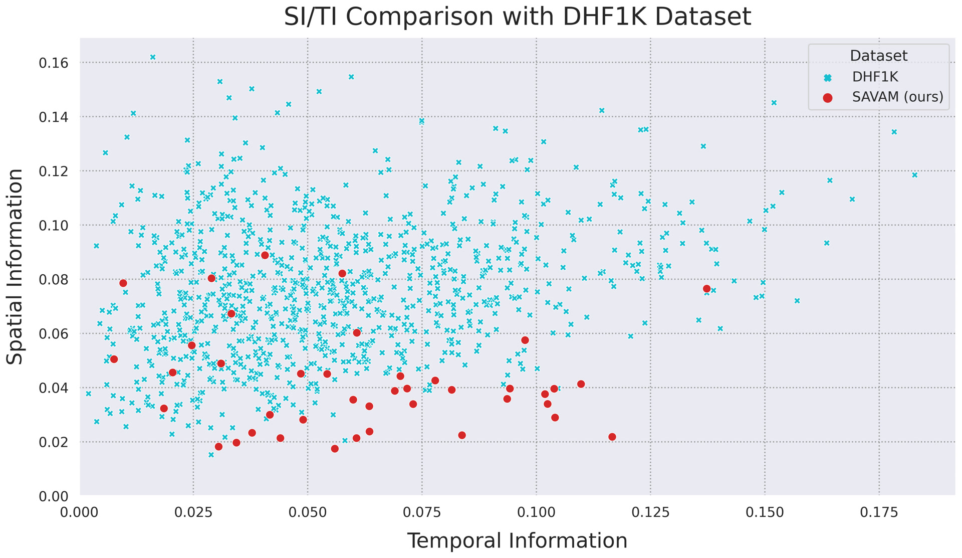
According to the graph, we can conclude that our dataset represents a domain of a different distribution with a diverse amount of movement on evenly spaced scenes. For comparison, we used the VQMT^[1] implementation of SI/TI metrics.

Metrics

Some articles have several variants of models to use, which differ in varying training datasets or architectures.
We hide these similar models by default, and you can view them using checkboxes.

We compute 3 metrics using Ground Truth Gaussians: Similarity (SIM), Linear Correlation Coefficient (CC)
and Kullback-Leibler divergence (KLDiv).
Also, we compute 2 metrics using Ground Truth fixations: Normalized Scanpath Saliency (NSS)
and Area Under the Curve — Judd (AUC Judd): evaluates a saliency map’s predictive power by how many ground truth fixations it captures in successive level sets.
In visualization and leaderboard, we sort models by the SIM metric, as by the basic metric for comparing video saliency prediction models.

We run saliency models on NVIDIA GTX 1060. Usually, saliency models utilize only GPU for neural network inference, but some also use CPU. We run saliency algorithms on Intel Core i5-7300HQ @ 2.50GHz. All models were tested on Linux.

Domain Adaptation

Saliency maps predicted by various visual-attention models can be significantly improved using sequences of simple postprocessing transformations: brightness correction and blending with the Center Prior.

The relevance of brightness correction is explained by the need to bring the obtained saliency maps to one form in the sense of the parameters of blurring fixations into Gaussians. Such a difference may manifest itself simply because different models used different ways of blurring Ground Truth fixations for training (although the data itself could be the same).
Thus, brightness correction adapts the size of domain predictions. Blending with Center Prior adapts the shape and location of domain predictions, giving the desired predictions the appearance of a Gaussian distribution and centering their location.

The need to use domain adaptation can be justified by differences in the average Gaussians of some other popular datasets:

For our evaluation, we used a method^[2] that for any saliency model can find the exact globally optimal blending weight and brightness-correction function simultaneously in terms of MSE.

Let \(\textbf{SM}^i\) and \(\textbf{GT}^i\) be the respective predicted and Ground Truth saliency maps for the \(i^\text{th}\) frame, and let \(\textbf{CP}\) be a precomputed Center Prior image. The blending weight is denoted by \(\beta\), and \(p \in \mathbb{R}^2\) is the pixel position. The cost function is then \[C(\beta,\, M) = \sum_{i,\, p} (M(\textbf{SM}^i_p) + \beta\,\textbf{CP}_p - \textbf{GT}^i_p)^2,\] where \(M : \mathbb{R}^+ \to \mathbb{R}^+\) is the brightness-correction function. Since we store saliency maps as 8-bit images, we can represent this function by the vector \(\textbf{m} \in \mathbb{R}^N\), \(N = 256\), such that \(M(s) = \textbf{m}_s \in \mathbb{R}^+\) for any saliency value \(s \in \mathbb{N}^+\), with \(s < N\). Then we can consider \(C\) to be the quadratic function of real-valued arguments \(\beta\) and \(\textbf{m}\), so the solution of the following quadratic programming problem should yield the optimal parameter values: \[(\beta,\, \textbf{m}) = \underset{0 < \textbf{m}_i < \textbf{m}_{i+1}}{\underset{\beta > 0}{\operatorname{arg min}}} \sum_{i,\, p} (\textbf{m}_{\textbf{SM}^i_p} + \beta\,\textbf{CP}_p - \textbf{GT}^i_p)^2.\] The constraints guarantee that the brightness-correction function \(\textbf{m} \in \mathbb{R}^N\) is monotone. This task has a canonical matrix form: \[(\beta,\, \textbf{m}) = \underset{0 < \textbf{x}_i < \textbf{x}_{i + 1},\, i > 1}{\underset{\textbf{x}_1 > 0}{\operatorname{arg min}}} \frac{1}{2}\textbf{x}^T\textbf{Hx} + \textbf{f}^T\textbf{x} + c,\] where \(\textbf{x} = (\beta,\, \textbf{m}) \in \mathbb{R}^{N + 1}\) contains the target parameters; matrix \(\textbf{H} \in \mathbb{R}^{(N + 1) \times (N + 1)}\), vector \(\textbf{f} \in \mathbb{R}^{N + 1}\) and scalar \(c\) define the optimization task. \(\textbf{H}\) is a Hermitian sparse matrix containing nonzero elements only in the first row, first column, and main diagonal. Moreover, \(\textbf{H}\) is a positive-definite matrix, so the quadratic programming task is convex and easily solved using any one of numerous approaches (we use the interior-point method).
The implementation of metrics calculating and domain adaptation is available at our github.

Subscribe to this benchmark's updates using the form and get notified when the paper will be available.

References

1. MSU Video Quality Measurement Tool
2. V.Lyudvichenko, M.Erofeev, Y.Gitman, and D.Vatolin, “A semiautomatic saliency model and its application to video compression,” in IEEE International Conference on Intelligent Computer Communication and Processing (ICCP), 2017, pp. 403–410