Evaluation methodology of MSU Video Super-Resolution Benchmark: Detail Restoration
You can read the Methodology below or download the presentation in pdf format
here.
You also can see it in
Google Slides here.
Problem definition
Super-Resolution is the process of calculating high-resolution samples from their low-resolution counterparts. Trends in quality assessment of upscaled videos and images are favoring estimation of statistical naturalness in combination with fidelity. But restoration fidelity is much more important than statistical naturalness for some tasks. Some VSR methods may produce the wrong digit or an entirely different face. Whether a method’s results are trustworthy depends on how well it restores truthful details. Our benchmark is aimed to find the best algorithms for the restoration of real details during Video Super Resolution processing.
Dataset
Content types
To analyze a VSR model’s ability to restore real details, we built a test stand containing patterns that are difficult for video restoration (Figure 1).
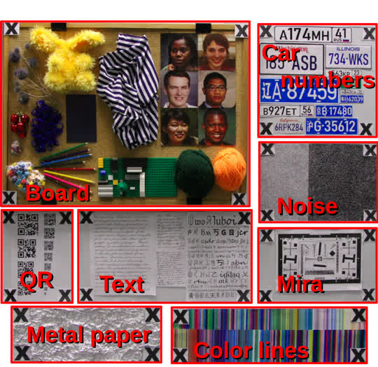
Figure 1. The test-stand of the benchmark.
To calculate metrics for particular content types
and to verify how a model works with different inputs,
we divide each output frame into parts by detecting
crosses:
Part 1. “Board” includes a few small objects and photos of human faces*. Our goal is to obtain results for the model operating on textures with
small details. The striped fabric and balls of
yarn may produce a Moire pattern (Figure 2).
Restoration of human faces is important for
video surveillance.
Part 2. “QR” comprises multiple QR codes of differing sizes; the aim is to find the size of the
smallest recognizable one in the model’s output frame. A low-resolution frame may blend
QR-code patterns, so models may have difficulty restoring them.
Part 3. “Text” includes two kinds: handwritten and
typed. Packing all these difficult elements into
the training dataset is a challenge, so they are
each new to the model as it attempts to restore
them.
Part 4. “Metal paper” contains foil that was vigorously crumpled. It’s an interesting example
because of the reflections, which change periodically between frames.
Part 5. “Color lines” is a printed image with numerous
thin color stripes. This image is difficult because thin lines of similar colors end up mixing in low-resolution frames.
Part 6. ‘License-plate numbers” consists of a set of
car license plates of varying sizes from different countries**. This content is important for
video surveillance and dashcam development
Part 7. “Noise” includes difficult noise patterns. Models cannot restore real ground-truth noise, and
each one produces a unique pattern
Part 8. “Resolution test chart” contains a resolution test chart with
patterns that are difficult to restore: a set of
straight and curved lines of differing thicknesses and directions
*Photos were generated by [1].
**The license-plate numbers are generated randomly and printed on paper.
Figure 2. Example of a Moire pattern on the “Board”.
Motion types
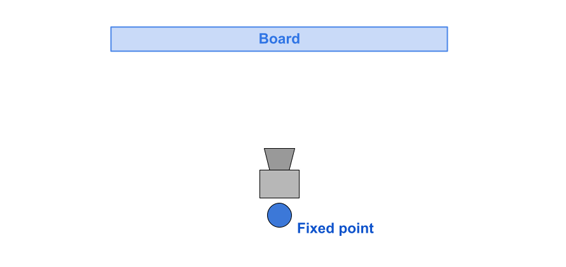
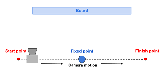
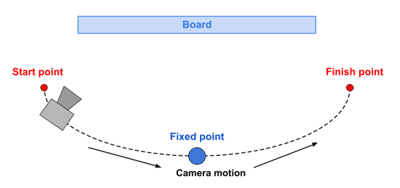
The dataset includes three videos with different types of motion:
- Hand tremor — video shooting from the fixed point without a tripod (the photographer holds the camera in his hands). Because of the natural tremor of hands, there is a random small motion in frames
- Parallel motion — the camera is moving from side to side in parallel with test-stand
- Rotation — the camera is moving from side to side in a half-circle
Technical characteristics of the camera
We captured the dataset using a Canon EOS 7D
camera. We quickly took a series of 100 photos and
used them as a video sequence. The shots were from
a fixed point without a tripod, so the video contains
a small amount of random motion. We stored the
video as a sequence of frames in PNG format, converted from JPG. The camera’s settings were:
ISO – 4000
aperture – 400
resolution – 5184x3456
Dataset preparation
- Source video has a resolution of 5184x3456 and was stored in the sRGB color space. Each video’s length is 100 frames.
- Ground-truth. Each video was degraded by bicubic interpolation to generate a GT of resolution 1920x1280. This step is essential because many open-source models lack the code to process a large frame; processing large frames is also time consuming.
- Then input video was degraded from GT in two ways: bicubic interpolation (BI) and Downsamlping after Gaussian Blurring (BD).
Noise input
To verify how a model works with noisy data, we prepared noise counterparts for each input video. To generate realistic noise, we use python implementation [2]
of the noise model proposed in CBDNet by Liu et al [3]. We need to set two parameters: one for the Poisson part of the noise and another for the Gauss part of
the noise.
To estimate the level of real noise in our camera, we set a camera on a tripod and capture a sequence of 100 frames from a fixed point. Then we average the sequence
to estimate a clean image. Thus we gain hundred of real noise examples. Then we chose parameters for generated noise so that the distributions of generated and real
noise are similar (see Figure 3). Our parameters choice: sigma_s = 0.001, sigma_c = 0.035.
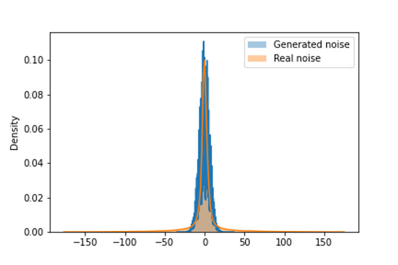
Figure 3. The distribution of real and generated noise.
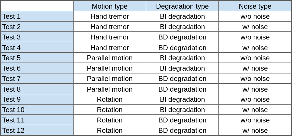
Finally, we have 12 tests:
Metrics
PSNR
PSNR – commonly used metric based on pixels’ similarity. We noticed that a model, trained on one degradation type and tested on another type, can generate frames with a global shift relative to GT (see Figure 4). Thus we checked integer shifts from [-3,3] in both axes and choose the shift with maximal PSNR value. This maximal value is considered as a metric result in our benchmark.
Figure 4. On the left: The same crop from the model’s output and GT frame.
On the right: PSNR visualization for this crop.
We chose PSNR-Y because it’s more efficient than PSNR-RGB. Meanwhile, a correlation between these metrics is high. For metric calculation, we use the implementation from skimage.metrics[4]. A higher metric value indicates better quality. The metric value for GT is infinite.
SSIM
SSIM – another commonly used metric based on structure similarity. A shift of frames can influence this metric too. Thus we tried to find the optimal shift similarly to PSNR calculation and noticed that optimal shifts for these metrics can differ, but not more than 1 pixel in any axis. Because SSIM has large computational complexity, we decided to find optimal shift not among all shifts, but near with optimal shift for PSNR (in a distance of 1 pixel in any axis). We calculate SSIM on the Y channel of the YUV color space. For metric calculation, we use the implementation from skimage.metrics[5]. A higher metric value indicates better quality. The metric value for GT is 1.
ERQAv1.0
ERQAv1.0 (Edge Restoration Quality Assessment, version 1.0) estimates how well a model has restored edges of the high-resolution frame. Firstly, we find edges in both output and GT frames. To do it we use OpenCV implementation[6] of the Canny algorithm[7]. A threshold for the initial finding of strong edges is set to 200. And a threshold for edge linking is set to 100. These coefficients allow to highlight edges of all subjects even of small sizes but skip lines, which are not important (see Figure 5).
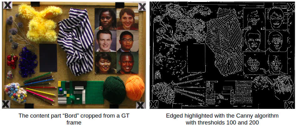
Figure 5. An example of edges, highlighted by the chosen algorithm
Then we compare these edges by using F1-score. To compensate a one-pixel shift of edge, which is not essential for human perception of objects, we consider as true-positive pixels of output’s edges, which are not in edges of GT but are near (on the difference of one pixel) with the edge of GT(see Figure 6). A higher metric value indicates better quality. The metric value for GT is 1.
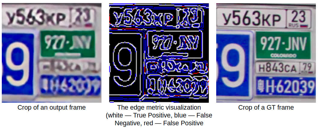
Figure 6. Visualization of F1-score, used for edges comparison
QRCRv1.0
QRCRv1.0 (QR-Codes Restoration, version 1.0) finds the smallest size (in pixels) of QR-code, which can be detected in output frames of a model. To project metric values on [0,1], we consider a relation of the smallest QRs’ sizes for GT and output frame (see Figure 7). If in the model’s result we can’t detect any QR-code, the metric value is set to 0. A higher metric value indicates better quality. The metric value for GT is 1.
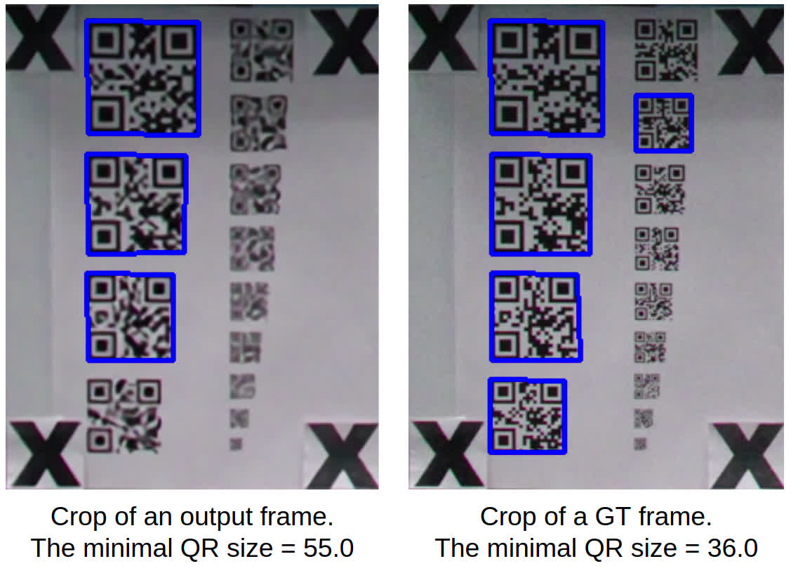
Figure 7. Example of detected crosses in output and GT frame.
The metric value for the output frame is 0.65
CRRMv1.0
CRRMv1.0 (Colorfullness Reduced-Reference Metric, version 1.0) – calculate colorfullness* in both frames and compare them. To calculate colorfullness we
use metric, proposed by Hasler et al.[8]. Comparison of colorfullness levels is performed as a relation between colorfullness in GT frame and output frame.
Then to project metric on [0,1] and penalize both increasing and decreasing of colorfullness, we take the absolute difference between 1 and the relation and
then subtract it from 1. A higher metric value indicates better quality. The metric value for GT is 1.
*Colorfulness measures how colorful an image is: if it’s bright and has a lot of different colors.
Metrics accumulation
Because each model can work differently on different content types, we consider metric values not only on full-frame but also on parts with different content.
To do this we detect crosses in frames and calculate coordinates of all parts from them.
Crosses in some frames are distorted and cannot be detected. Thus we choose keyframes, where we can detect all crosses and calculate metrics only on these
keyframes. We noticed that metrics values on these keyframes are highly correlated and choose the mean of values through keyframes as a final metric value
for each test case.
Subjective comparison
We cut the sequences to 30 frames and converted them to 8 frames per second (fps). This length allows subjects to easily consider details and decide which video is better. We then cropped from each video 10 snippets that cover the most difficult patterns for restora- tion and conducted a side-by-side pairwise subjective evaluation using the Subjectify.us service, which enables crowd-sourced comparisons.
To estimate information fidelity, we asked participants in the subjective comparison to avoid choosing the most beautiful video, but instead choose the one that shows better detail restoration. Participants are not experts in this field thus they do not have professional biases. Each participant was shown 25 paired videos and in each case had to choose the best video (“indistinguishable” was also an option). Each pair of snippets was shown to 10-15 participants until confidence interval stops changing. Three of pairs for each participant are for verification, so the final results exclude their answers. All other responses* from 1400 successful participants are used to predict subjective scores using the Bradley-Terry. *Answers to verification questions are not included in the final result.
The computational complexity of models
We tested each model using NVIDIA Titan RTX and measured runtime on the same test sequence:
- Test case — parallel motion + BD degradation + with noise
- 100 frames
- Input resolution — 480×320
References
- https://thispersondoesnotexist.com
- https://github.com/yzhouas/CBDNet_ISP
- Shi Guo, Zifei Yan, Kai Zhang, Wangmeng Zuo and Lei Zhang, "Toward Convolutional Blind Denoising of Real Photographs," 2019 IEEE/CVF Conference on Computer Vision and Pattern Recognition (CVPR), 2019, pp. 1712-1722, doi: 10.1109/CVPR.2019.00181.
- https://scikit-image.org/docs/stable/api/skimage.metrics.html#skimage.metrics.peak_signal_noise_ratio
- https://scikit-image.org/docs/stable/api/skimage.metrics.html#skimage.metrics.structural_similarity
- https://docs.opencv.org/3.4/dd/d1a/group__imgproc__feature.html#ga04723e007ed888ddf11d9ba04e2232de
- https://en.wikipedia.org/wiki/Canny_edge_detector
- David Hasler and Sabine Suesstrunk, "Measuring Colourfulness in Natural Images," Proceedings of SPIE - The International Society for Optical Engineering, 2003, volume 5007, pp. 87-95, doi: 10.1117/12.477378.
-
MSU Benchmark Collection
- Super-Resolution Quality Metrics Benchmark
- Video Colorization Benchmark
- Video Saliency Prediction Benchmark
- LEHA-CVQAD Video Quality Metrics Benchmark
- Learning-Based Image Compression Benchmark
- Super-Resolution for Video Compression Benchmark
- Defenses for Image Quality Metrics Benchmark
- Deinterlacer Benchmark
- Metrics Robustness Benchmark
- Video Upscalers Benchmark
- Video Deblurring Benchmark
- Video Frame Interpolation Benchmark
- HDR Video Reconstruction Benchmark
- No-Reference Video Quality Metrics Benchmark
- Full-Reference Video Quality Metrics Benchmark
- Video Alignment and Retrieval Benchmark
- Mobile Video Codecs Benchmark
- Video Super-Resolution Benchmark
- Shot Boundary Detection Benchmark
- The VideoMatting Project
- Video Completion
- Codecs Comparisons & Optimization
- VQMT
- MSU Datasets Collection
- Metrics Research
- Video Quality Measurement Tool 3D
- Video Filters
- Other Projects