The Methodology of the CrowdSAL Dataset and Benchmark
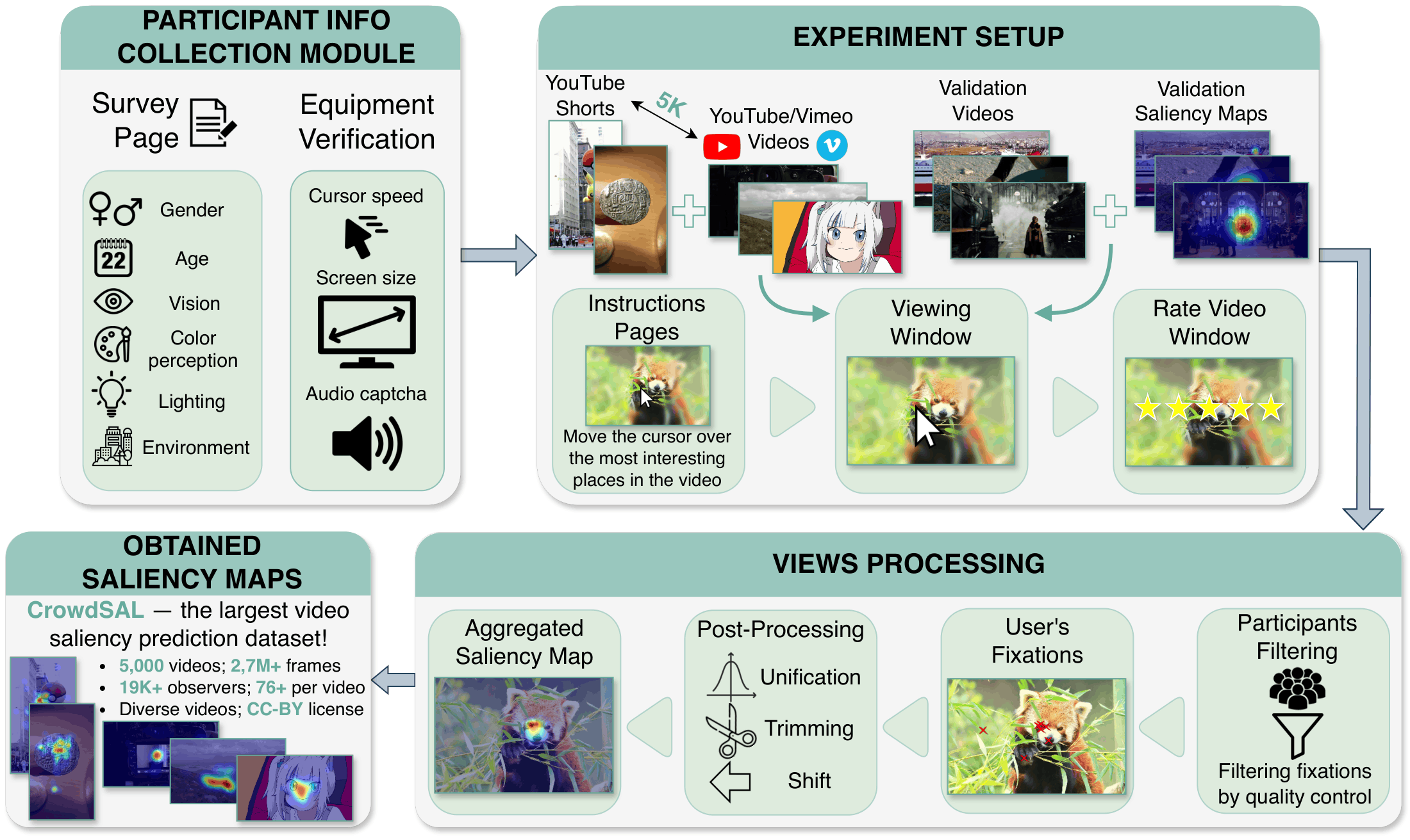
Proposed methodology pipeline for collecting saliency maps via crowdsourcing.
Data Collection
From YouTube, Shorts and Vimeo, we retained only videos released under CC-BY or CC0 licenses. For Vimeo, we additionally required a minimum bitrate of 20 Mbps. Across all sources, only videos with at least Full HD resolution were kept. Since many videos were longer than necessary, we extracted the central 20-second segment to avoid non-representative content such as intros or end credits. All selected videos were transcoded with libx264 at CRF 16, 30 FPS, and Full HD resolution. Subtitles and data streams were removed from all videos. Although the source videos shared the same aspect ratio, their resolutions varied, so all outputs were standardized to either 1920×1080 or 1080×1920. Audio was normalized according to EBU R128 and transcoded to stereo AAC at 256Kbps. To reduce bias toward particular spatial structures or motion patterns, we performed content selection by clustering videos using Spatial Information (SI) and Temporal Information (TI), following ITU-T P.910[1] . As SI/TI are widely used measures of multimedia content complexity, this helped ensure broader coverage of spatial detail and temporal dynamics. For clustering feature extraction, we used the VQMT[2] implementation of SI/TI metrics.
From YouTube, Shorts, and Vimeo, we retained only videos released under CC-BY or CC0 licenses. For Vimeo, we additionally required a minimum bitrate of 20 Mbps. Across all sources, only videos with at least Full HD resolution were kept. Since many videos were longer than necessary, we extracted the central 20-second segment to avoid non-representative content such as intros or end credits. All selected videos were transcoded with libx264 at CRF 16, 30 FPS, and Full HD resolution. Subtitles and data streams were removed from all videos. Although the source videos shared the same aspect ratio, their resolutions varied, so all outputs were standardized to either 1920×1080 or 1080×1920. Audio was normalized according to EBU R128 and transcoded to stereo AAC at 256 Kbps. To reduce bias toward particular spatial structures or motion patterns, we performed content selection by clustering videos using Spatial Information (SI) and Temporal Information (TI), following ITU-T P.910[1]. As SI/TI are widely used measures of multimedia content complexity, this helped ensure broader coverage of spatial detail and temporal dynamics. For the features used in clustering, we used the VQMT[2] implementation of SI/TI metrics.
Our dataset consists of 5,000 clips. Each video was viewed by more than 75 observers. The final saliency map was estimated as a Gaussian mixture with centers at the fixation points. We set the Gaussian standard deviation to 57.6 pixels. Under standard viewing conditions, with a viewing distance of 60 cm and a screen width of 35 cm / 1920 px, this value corresponds to approximately 1 degree of visual angle. The frame saliency maps were also transcoded with libx264 at CRF 0, 30 FPS, 10-bit luminance depth, and Full HD resolution to match the source videos.
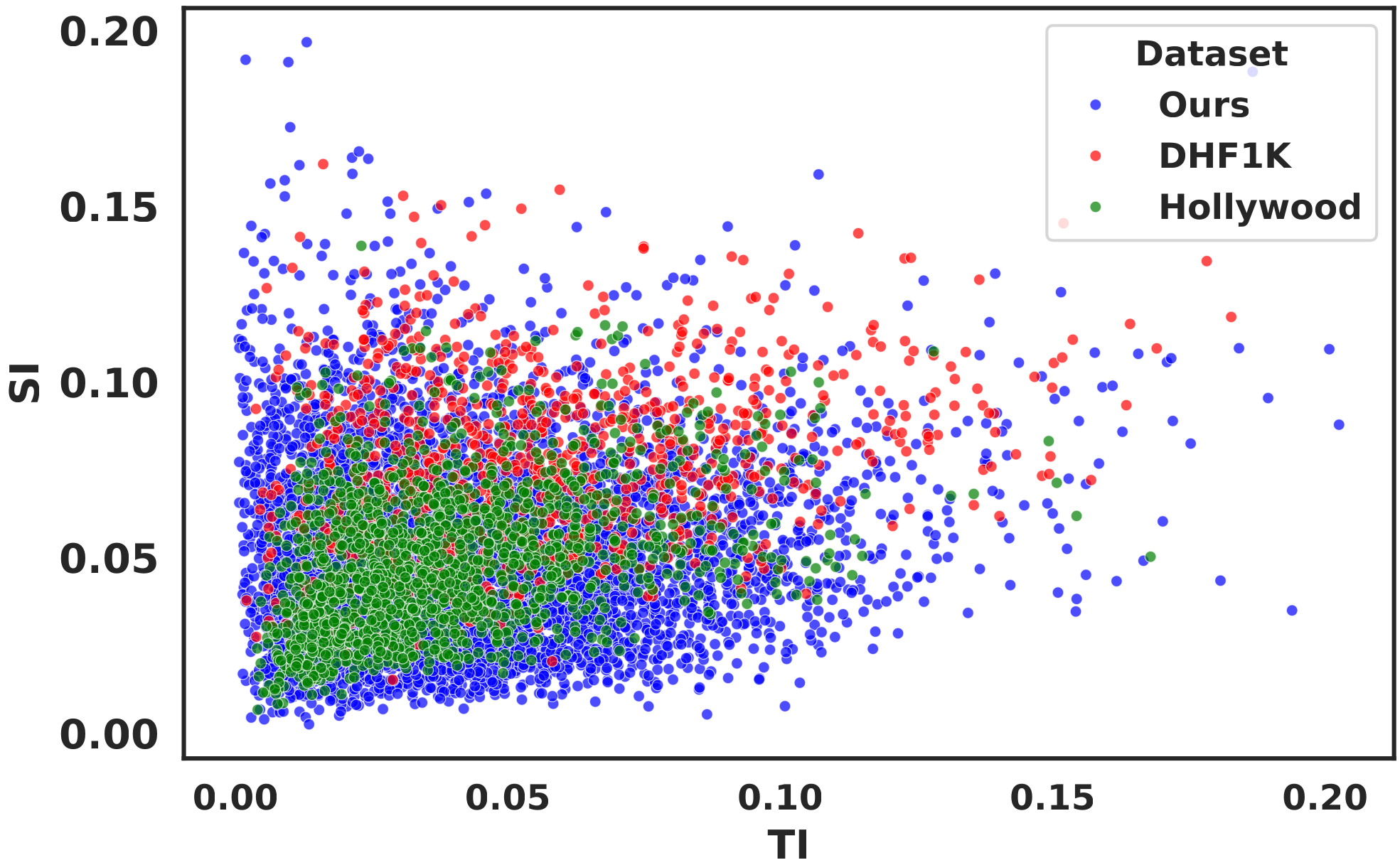
As shown in the figure, our CrowdSAL dataset has a more diverse distribution of motion and spatial information values than the DHF1K and Hollywood-2 datasets, which contain 1,000 and 1,707 videos, respectively. For this comparison, we used SI/TI metrics to characterize the spatial and temporal complexity of the datasets.
Saliency Metrics[3]
The metric implementations used in this work are available on our GitHub.
We compute two metrics using Ground Truth gaussians: the Linear Correlation Coefficient (CC) and Similarity (SIM). \[ \begin{aligned} &\mathrm{CC}(P,Q^{D}) = \frac{\sigma(P,Q^{D})}{\sigma(P) \times \sigma(Q^{D})} \\[4pt] &\mathrm{SIM}(P,Q^{D}) = \sum_i \min(P_i,Q^{D}_i), \quad \sum_i P_i = \sum_i Q^{D}_i = 1. \end{aligned} \] We also compute two metrics using Ground Truth fixations: Normalized Scanpath Saliency (NSS) and Area Under the Curve by Judd (AUC Judd). AUC Judd evaluates a saliency map's predictive power by measuring how many Ground Truth fixations it captures in successive level sets. \[ \begin{aligned} &\mathrm{NSS}(P,Q^{B}) = \frac{1}{N}\sum_{i} \bar P_i \times Q^{B}_i, \quad \bar P = \frac{P-\mu(P)}{\sigma(P)}, \quad N=\sum_i Q^{B}_i. \\[2pt] &\mathrm{AUC\text{ }Judd}(S,F) = \sum_{k=1}^{K-1} \frac{\mathrm{TPR}_{k+1}+\mathrm{TPR}_k}{2}\, \bigl(\mathrm{FPR}_{k+1}-\mathrm{FPR}_k\bigr), \\[2pt] &\mathrm{TPR}_k = \frac{\sum_i \mathbf{1}[P_i \ge \tau_k]\; Q^{B}_i}{\sum_i Q^{B}_i}, \quad \mathrm{FPR}_k = \frac{\sum_i \mathbf{1}[P_i \ge \tau_k]\,(1-Q^{B}_i)} {\sum_i (1-Q^{B}_i)}. \end{aligned} \]
Notation:
- \(i\) — pixel index,
- \(P\) — predicted saliency map,
- \(Q^{B}_i \in \{0,1\}\) — binary Ground Truth fixation map,
- \(Q^{D}_i \ge 0\) — continuous Ground Truth saliency map,
- \(\mu(M)\) — mean value of \(M\),
- \(\sigma(M)\) — standard deviation of \(M\),
- \(\sigma(A,B)\) — covariance between \(A\) and \(B\),
- \(\mathbf{1}[\cdot]\) — indicator function,
- \(K\) — number of distinct thresholds,
- \(\{\tau_k\}_{k=1}^K\) — sorted distinct values of \(P\).
Optimal Sigmas Selection
The balance between the visible foreground region and the blur applied to the background affects how strongly participants are encouraged to move the cursor. We conducted a greedy search on the validation benchmark, varying the foveal foreground diameter of the visible region \(\sigma_{fg}\), and the background blur level as the Gaussian standard deviation \(\sigma_{bg}\), both as a percentage of the screen width. In total, we tried 17 combinations. All values are computed relative to the participant's screen width. The mean CC, SIM, and NSS values in the table below indicate that the optimal setting is \(\sigma_{bg} = 0.5\) and \(\sigma_{fg} = 20\). The error intervals are defined as standard deviations.
Participants Validation
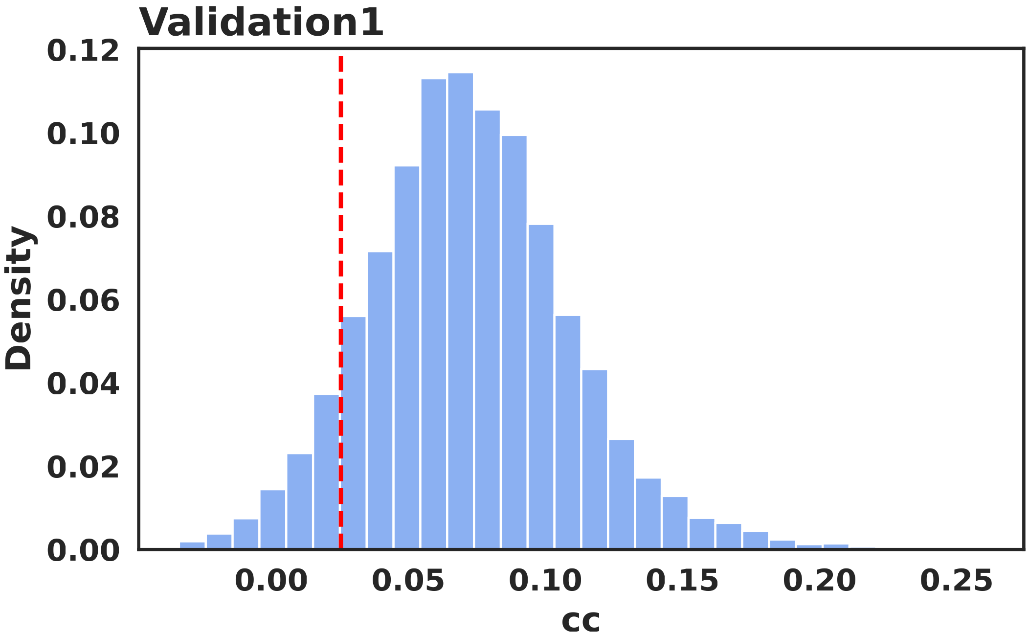
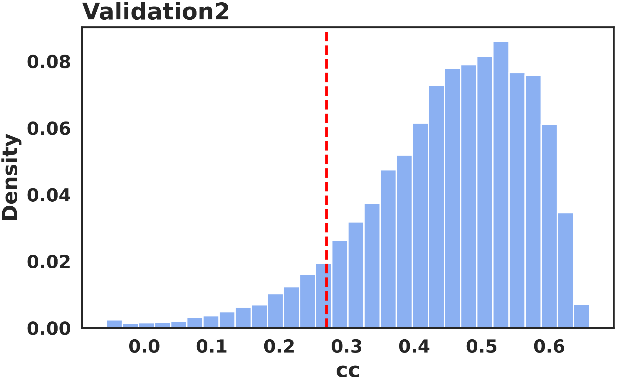
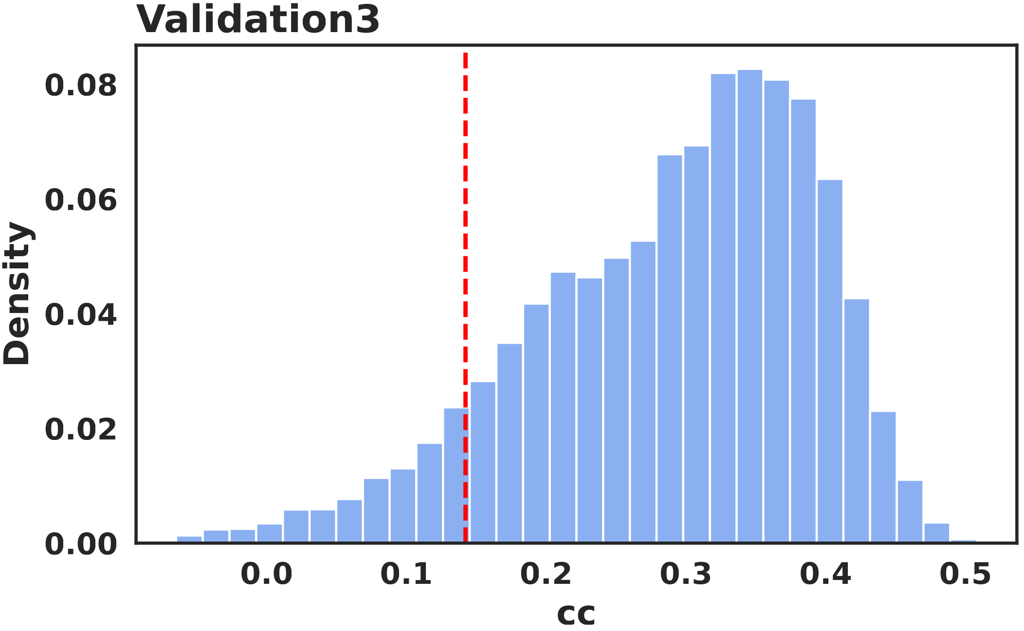
The first post-filtering stage uses honeypot videos. These clips were selected as the three most challenging cases for our methodology. Using the validation benchmark, we determined quality thresholds for these videos and excluded participants whose responses fell below them. The distributions of the mean CC on each individual honeypot video show that the mouse-based saliency signal remains aligned with the original attention pattern after filtering. These participants were still compensated, but their data were removed from the final dataset. Filtering on the validation videos retained 19,632 participants (~80%).
Frequency Analysis
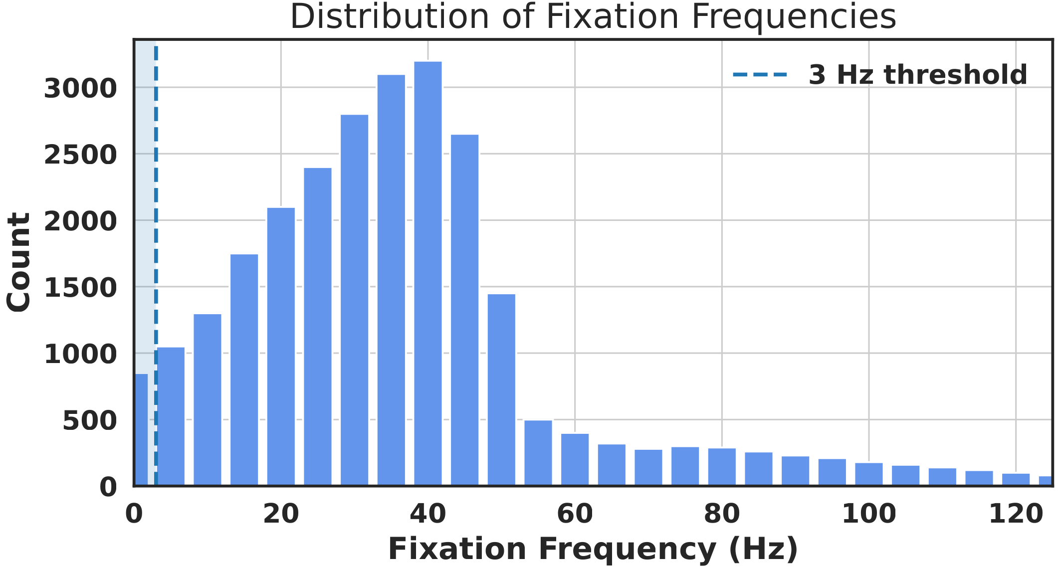
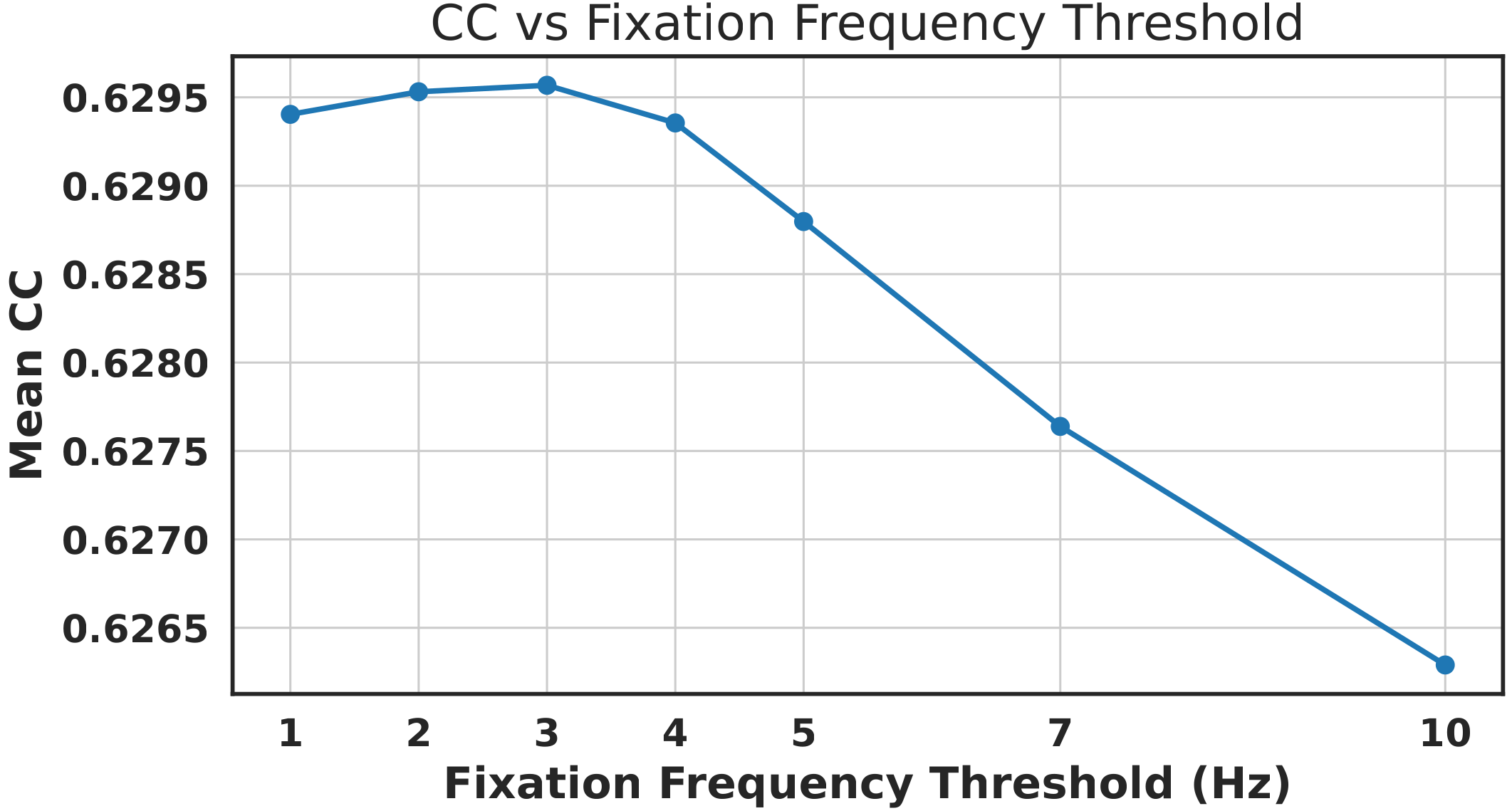
The second post-filtering stage is based on mouse movement frequency. The rationale is that a participant may appear to be watching the video without actively interacting with the mouse. The distribution shows that most accepted views fall well below 100 Hz. We evaluated several frequency thresholds on the validation benchmark and found that 3 Hz provides the best trade-off. We therefore discard views below 3 Hz and normalize the remaining trajectories to 100 Hz using linear interpolation. Frequency filtering passed 381,960 successful views (~93.7%).
Dataset Statistics
The average video length in the CrowdSAL dataset after all transformations is 553 frames (~18.4 seconds). The average time required to complete the crowdsourcing task is less than 15 minutes. In the graphs below, we report statistics for participants who successfully passed all filtering stages.
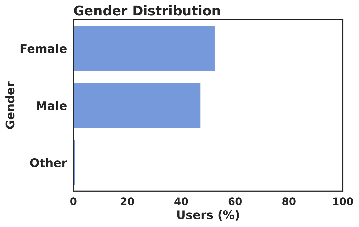
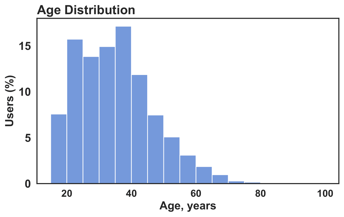
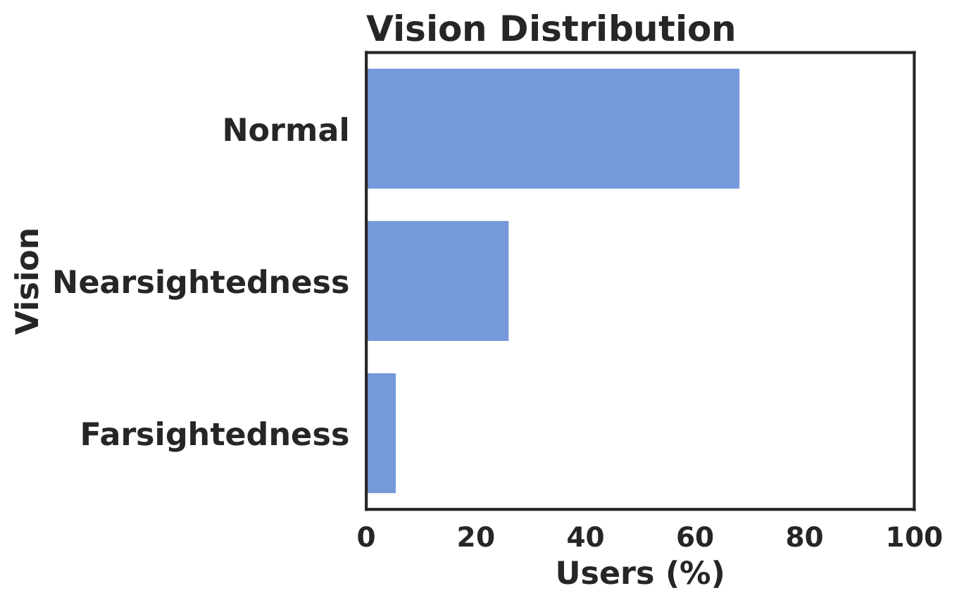
The accepted participant pool is not dominated by a single gender group. The study primarily reflects adult viewing behavior. Most accepted participants reported normal vision.
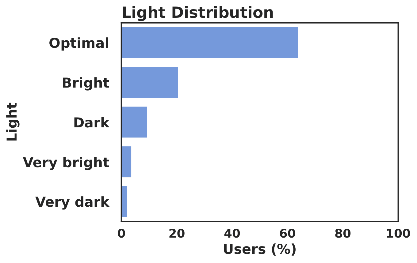
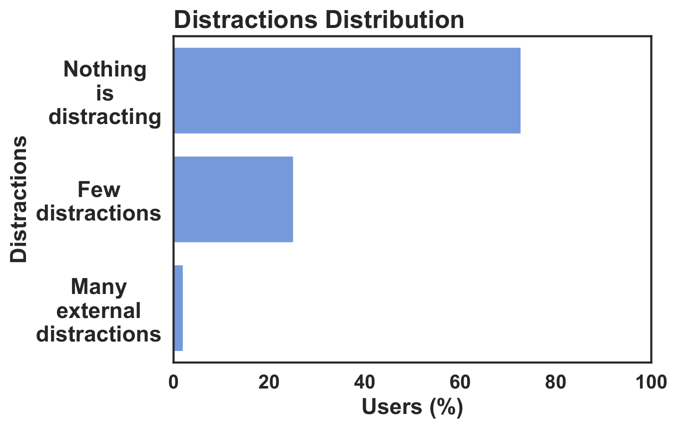
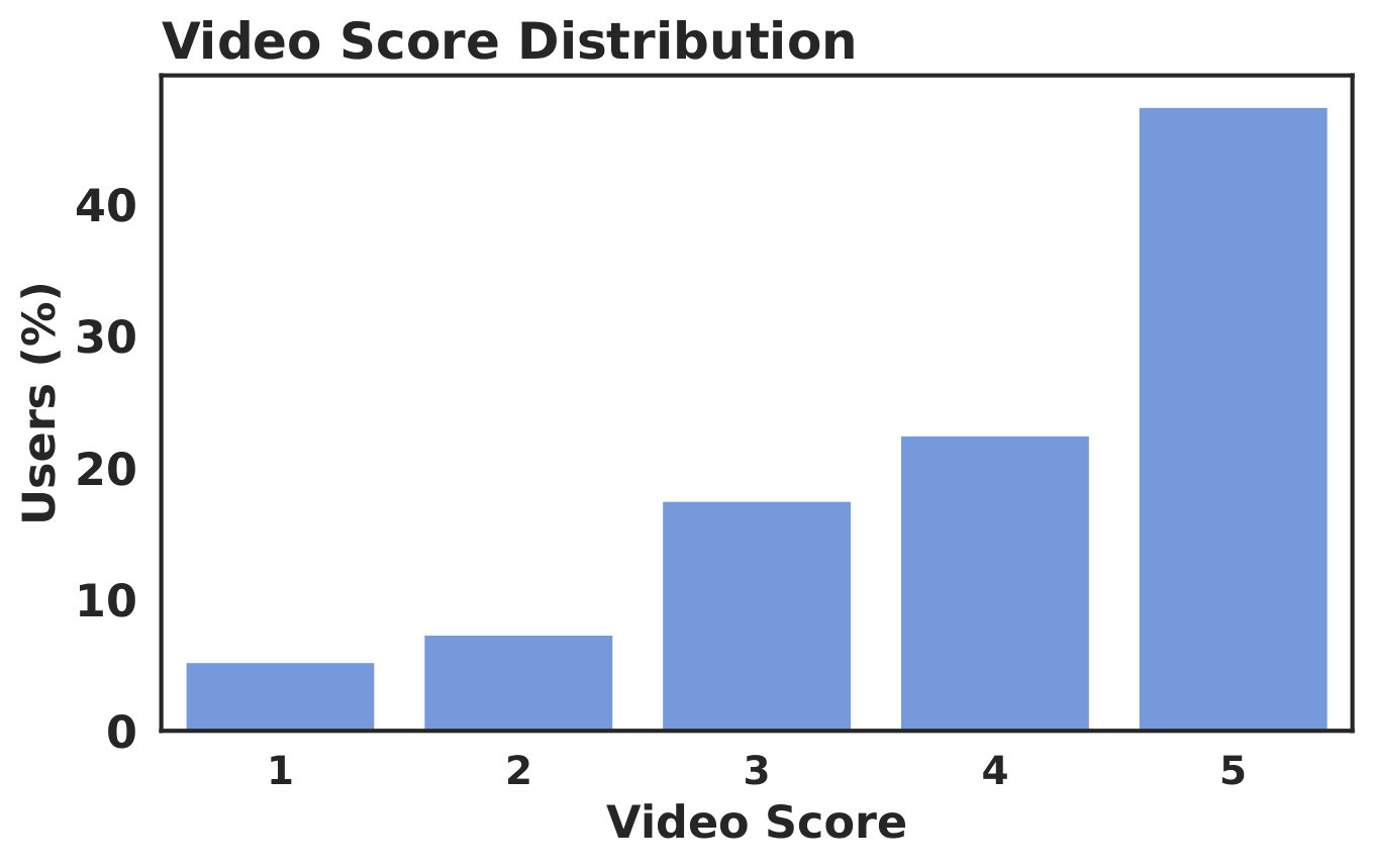
The recordings were collected under realistic everyday lighting conditions. The accepted sessions cover a variety of viewing setups. The 1-5 star ratings were collected from participants as post-task feedback after they finished each video.
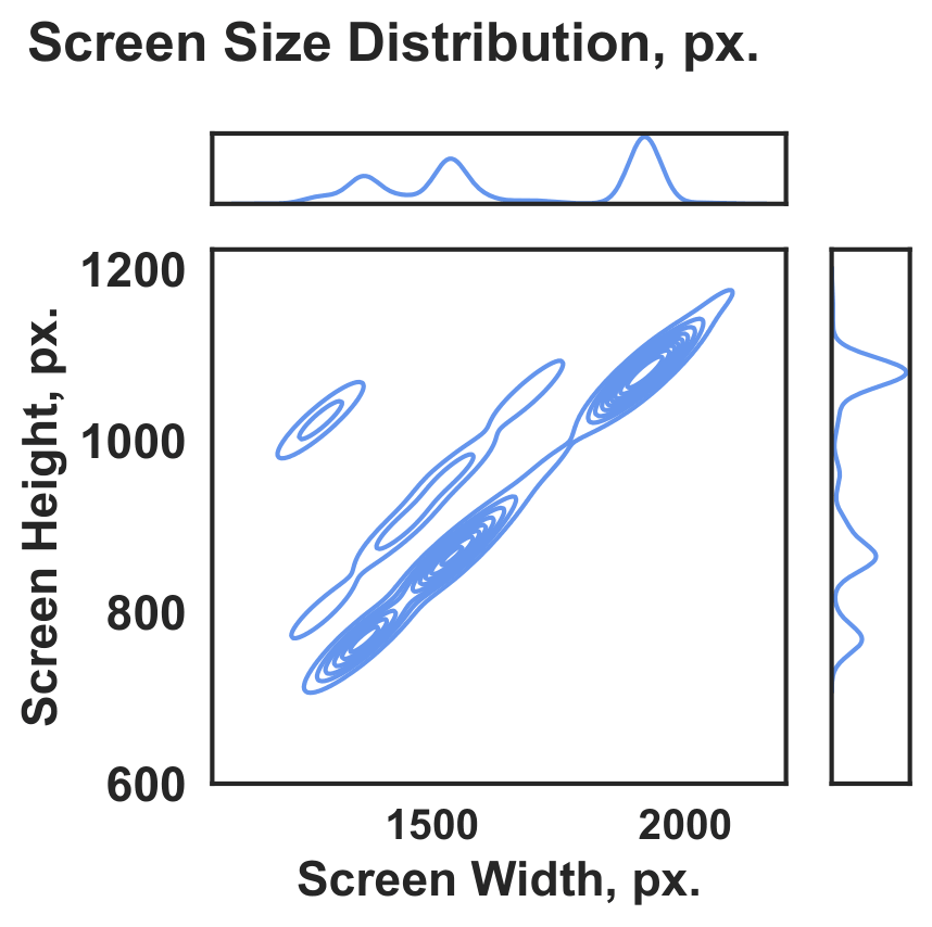
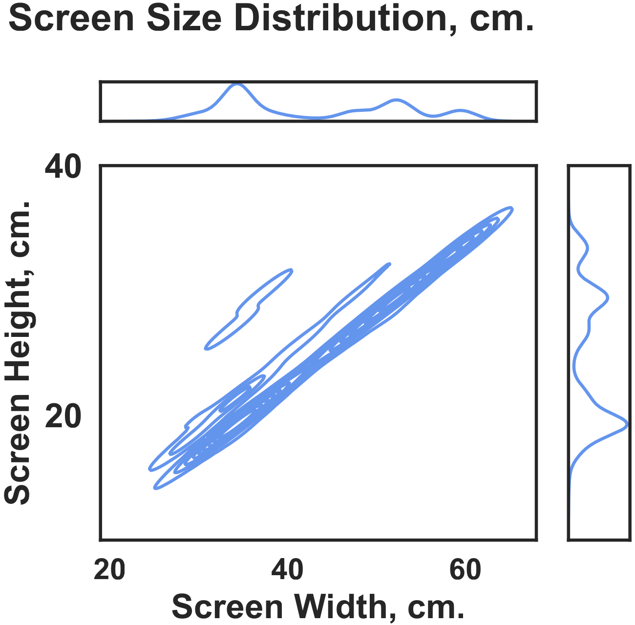
The accepted data span a broad range of screen resolutions and physical screen sizes. The most common setup was a 1920×1080 px display with a 34×19 cm screen.
Validation With Automatic Models
The table below compares model generalization across external saliency benchmarks using CC, SIM, NSS, and AUC Judd. The Human Infinite row in the table below estimates the consistency ceiling by comparing one group of human annotations with another. For this estimate, the fixations in each video frame are split into two groups. The table shows that our method outperforms all automatic video saliency models in terms of CC, SIM, and NSS. Moreover, in terms of CC, our method is closer to Human Infinite than to the second-best automatic method. For SIM and NSS, our method remains noticeably closer to Human Infinite than to most automatic methods. This shows that the difference between our method and automatic methods is significant.
For the benchmark on the CrowdSAL dataset, we report model size (#Parameters) and FPS (frames per second) for all models, measured on a single NVIDIA TESLA A100 80GB GPU.
References
- International Telecommunication Union. 2008. Subjective video quality assessment methods for multimedia applications. ITU-T Recommendation P.910. ITU-T, Geneva, Switzerland. Approved 2008-04-06.
- MSU Video Quality Measurement Tool
- Zoya Bylinskii, Tilke Judd, Aude Oliva, Antonio Torralba, and Frédo Durand. 2018. What do different evaluation metrics tell us about saliency models? IEEE transactions on pattern analysis and machine intelligence 41, 3 (2018), 740–757.
-
MSU Benchmark Collection
- Super-Resolution Quality Metrics Benchmark
- Video Colorization Benchmark
- Video Saliency Prediction Benchmark
- LEHA-CVQAD Video Quality Metrics Benchmark
- Learning-Based Image Compression Benchmark
- Super-Resolution for Video Compression Benchmark
- Defenses for Image Quality Metrics Benchmark
- Deinterlacer Benchmark
- Metrics Robustness Benchmark
- Video Upscalers Benchmark
- Video Deblurring Benchmark
- Video Frame Interpolation Benchmark
- HDR Video Reconstruction Benchmark
- No-Reference Video Quality Metrics Benchmark
- Full-Reference Video Quality Metrics Benchmark
- Video Alignment and Retrieval Benchmark
- Mobile Video Codecs Benchmark
- Video Super-Resolution Benchmark
- Shot Boundary Detection Benchmark
- The VideoMatting Project
- Video Completion
- Codecs Comparisons & Optimization
- VQMT
- MSU Datasets Collection
- Metrics Research
- Video Quality Measurement Tool 3D
- Video Filters
- Other Projects